Viacheslav Shalisko blog

Сегодня я прослушал на Эхо Москвы передачу, в которой обсуждались жизненные обстоятельства россиян и заирагивалась тема их личного выбора, который на самом деле до сих пор существует. Я с этим совершенно согласен и тоже считаю что сейчас выбор может быть только личным, и многеюие его сделали, и я его сделал. Меня эта тема беспокоит, так как всё же существует некоторая этическая напряженность, связанная с этим выбором и всё же хочется знать мнение других людей об этом. Так вот, зная что жизненные обстоятельства россиян в настоящее время, и в ближайшем будущем являются неизменной данностью, являниями подобными вечной мерзлоте или северному сиянию, такой личный выбор делать проще.
На Эхо Москвы было ещё несколько ярких слов про северное сияние, но я их не стану повторять.

Mar 10, 2018

Visualization of paired Mann-Whitney U test for several variables in R

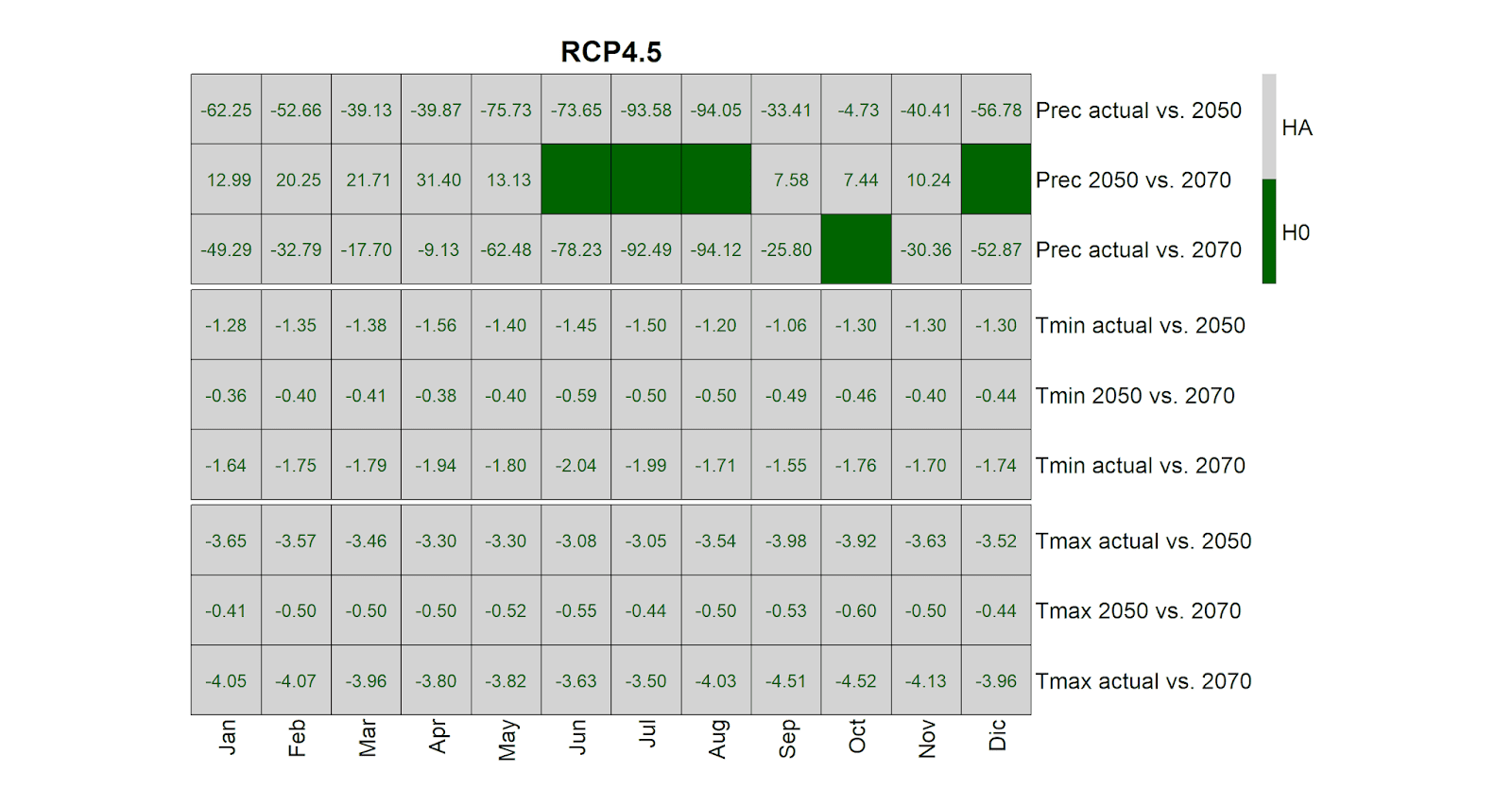
As a part of our recent research, we made several visualizations of variable comparizon. The boxplot gives good visual results, but the paired Mann-Whitney U test is required to access the statistical significance of differences. In order to visualize results of this test we us the following graphics:

The package pheatmap ver. 1.0.8 was found to be rather useful and flexible for visualization of such paired test data. Usually this package is used to make heatmaps with clusterization, but our choice is to adopt it to deal with binary data. Here is some code fragments used to perform the test and visualize it results.
The test itself is part of the following function:

compareMWT = function(x, y, test_title, alternative='two.sided') {
  wilcoxTest_result <- wilcox.test(x,y,
                        alternative=alternative,conf.int=TRUE)
  cat('Mann-Whitney test results for',test_title,"\n",sep=' ')
  if (wilcoxTest_result$p.value < 0.05) {
      cat('The H0 is rejected as p < 0.05, 
              the HA accepted (medians unequal)',"\n")
  } else {
      cat('The HA is rejected as p >= 0.05, 
              the H0 accepted (medians equal)',"\n")
  }  
  print(wilcoxTest_result)
}

Our data includes Magn_prec00, Magn_prec50, Magn_prec70 and similar variables as data to be compared. The month_list is month names vector. Test is called in cycle (12 months) for the desired combinations (pairs) of variables. Test results are stored in two matrices: one for binary output (the H0 is coded as 0 and the HA as 1), and another matrix is to store the estimation of centrality shift.

# true-false H0 vs. HA matrices
MWU_prec_RCP45_matrix <- matrix(nrow = 12, ncol = 3)

# location shift estimation matrices
MWU_prec_RCP45_matrix_s <- matrix(nrow = 12, ncol = 3)

for (i in 1:12) {
  my_test1 <- compareMWT(Magn_prec00[,i],Magn_prec50[,i],
    paste(month_list[i],'precipitation: actual vs. RCP4.5 2050'))
  my_test2 <- compareMWT(Magn_prec50[,i],Magn_prec70[,i],
    paste(month_list[i],'precipitation: RCP4.5 2050 vs. RCP4.5 2070'))
  my_test3 <- compareMWT(Magn_prec00[,i],Magn_prec70[,i],
    paste(month_list[i],'precipitation: actual vs. RCP4.5 2070'))

  if (my_test1$p.value < 0.05) {
    MWU_prec_RCP45_matrix[i,1] <- 1
    MWU_prec_RCP45_matrix_s[i,1] <- my_test1$estimate
  } else {
    MWU_prec_RCP45_matrix[i,1] <- 0
  }
  if (my_test2$p.value < 0.05) {
    MWU_prec_RCP45_matrix[i,2] <- 1
    MWU_prec_RCP45_matrix_s[i,2] <- my_test2$estimate    
  } else {
    MWU_prec_RCP45_matrix[i,2] <- 0
  }
  if (my_test3$p.value < 0.05) {
    MWU_prec_RCP45_matrix[i,3] <- 1
    MWU_prec_RCP45_matrix_s[i,3] <- my_test3$estimate    
  } else {
    MWU_prec_RCP45_matrix[i,3] <- 0
  }
}

The visualization in pheatmap is nice, but the labels of the x-axis are oriented 270° by default, to override this strange feature we use custom function, identical to draw_columns internal function of pheatmap, except the rotation rot = 90 and ajustment hjust = 1. The override works within session by assignInNamespace.

library(pheatmap)

draw_colnames_90 <- function(coln, gaps, ...) {
    coord = pheatmap:::find_coordinates(length(coln), gaps)
    x = coord$coord - 0.5 * coord$size
    res = grid:::textGrob(coln, x = x, 
          y = grid:::unit(1, "npc") - grid:::unit(3, "bigpts"), 
          vjust = 0.5, hjust = 1, rot = 90, gp = grid:::gpar(...))
    return(res)
}  

assignInNamespace(x="draw_colnames", 
          value="draw_colnames_90", ns=asNamespace("pheatmap"))

The visualization itself inslude dark green cells for cases where the H0 is acepted (no significant difference in medians), and light gray cells for cases of alternative hypothesis HA. The numbers within cells indicate the estimated median shift.

MWU_prec_RCP45_matrix_s <- format(MWU_prec_RCP45_matrix_s, 
                                        digits=2, nsmall=2)
MWU_tmin_RCP45_matrix_s <- format(MWU_tmin_RCP45_matrix_s, 
                                        digits=2, nsmall=2)
MWU_tmax_RCP45_matrix_s <- format(MWU_tmax_RCP45_matrix_s, 
                                        digits=2, nsmall=2)

pheatmap(rbind(t(MWU_prec_RCP45_matrix),
               t(MWU_tmin_RCP45_matrix),
               t(MWU_tmax_RCP45_matrix)), 
         display_numbers = rbind(
               t(MWU_prec_RCP45_matrix_s),
               t(MWU_tmin_RCP45_matrix_s),
               t(MWU_tmax_RCP45_matrix_s)),
         fontsize_number = 13, 
         number_color = 'darkgreen',
         color = c('darkgreen','lightgray'), 
         border_color = 'black', 
         cellwidth = 50, cellheight = 50,
         symm = FALSE, 
         cluster_rows = FALSE, 
         cluster_cols = FALSE,
         gaps_row = c(3,6),
         legend_breaks = c(0,0.25,0.5,0.75,1), 
         legend_labels = c('','H0','','HA',''),
         labels_col = month_list,
         labels_row = c('Prec actual vs. 2050',
          'Prec 2050 vs. 2070','Prec actual vs. 2070',
                        'Tmin actual vs. 2050',
          'Tmin 2050 vs. 2070','Tmin actual vs. 2070',
                        'Tmax actual vs. 2050',
          'Tmax 2050 vs. 2070','Tmax actual vs. 2070'),
         main = 'RCP4.5', fontsize = 16)

Mar 7, 2018

Puerto los Mazos Excursionismo

https://connect.garmin.com/modern/activity/2535490155#.WqA6HMnvxJE.google_plusone_share Читать дальше......

Feb 1, 2018

Безнадёжно

Приведу фрагмент из интервью Антона Красовского на Эхе Москвы (Разбор полёта) от 29.1.2018:
- ... Мы сегодня вспоминали о 90-х, которые некоторые характеризуют как время надежд... А сегодняшнее время, каким словом может быть охарактеризовано, спестя десяток лет?
А.К. - Безнадёжно, конечно. А у Вас есть надежда?
- Как-то стараюсь жить с этим чувством...
А.К. - У меня, например, нет. Я ещё раз говорю, я сейчас вижу огромное колличество людей, я слышу что они говорят, и я прекрасно понимаю, что у нескольких поколений здесь нет никакого будущего, абсолютно никакого. Они сами его профукали, они его сами разменяли, они сами свою свободу растоптали, они сделали всё, для того чтобы эта свобода, и это право на свободу были растоптаны, собственными сапогами. И они не заслужили права на свободу, они её не получат. Поэтому у нескольких поколений здесь нет никакой надежды. Но потом, возможно, начнётся возрождение.
- А будущее, в котором не осознаётся его отсутствие большинством, достойно ли оно наступать?
А.К. - Это сложный вопрос, потому что предполагает некоторую конечность человеческого объединения. Для большинства людей с которыми Моисей вышел из египетского плена будущее так и не наступило, но для великого народа оно явилось. Я уверен, что у великого русского народа это будущее есть, но у моего поколения, например, нет.

Я соглашаюсь с этим фрагментом А.К., учитывая данные прессы, результаты личных наблюдений 2017 года, и на основе очень интересной беседы с коллегой В.М. (знаменитым учёным), с которой мы недавно случайно оказались на соседних креслах в самолёте из Парижа в Петербург, и которая рассказала много интересного.

Jan 25, 2018

Дорогая бабушка, я и мы тебя всегда будем любить и помнить.

Дорогая бабушка, я и мы тебя всегда будем любить и помнить. Ты была такая! Ты так много сделала для меня, научила так многому! Все годы рядом с тобой были как чудо. Как жаль что тебя больше нет.

Jan 7, 2018

Hirosima @ SPb International Airport "Pulkovo"

Hirosima @ SPb International Airport "Pulkovo" Читать дальше......

Dec 12, 2017

Полезные рассуждения по поводу этики и межгендерных отношений.

Полезные рассуждения по поводу этики и межгендерных отношений.
https://youtu.be/Ec52pvOM76A Читать дальше......

Dec 3, 2017

¿Que mejor refleja estructura básica de consumo en una ciudad?

¿Que mejor refleja estructura básica de consumo en una ciudad? Los Starbucks es un "proxy" excelente, por l menos en caso de GDL. Читать дальше......

Jun 7, 2017

Multiple RStudio instances HOW-TO

Multiple RStudio instances HOW-TO
Brief guide to run multiple independent RStudio instances on the same machine. Sometimes it could be useful to run several RStudio scripts simultaneously. The standard RStudio 0.99.902 on Windows 10 machine do not allow such functionality, as the single R en...
http://vshalisko.blogspot.com/2017/06/multiple-rstudio-instances-how-to.html Читать дальше......

Multiple RStudio instances HOW-TO

Brief guide to run multiple independent RStudio instances on the same machine.

Sometimes it could be useful to run several RStudio scripts simultaneously. The standard RStudio 0.99.902 on Windows 10 machine do not allow such functionality, as the single R environment is linked to all instances of RStudio you can run. The solution I found is to install RStudio server on virtual machine (container) and use several copies of such container to be able to run several independent analysis.

The solution include several steps:

1) You should have Docker (www.docker.com) container manager installed on your Windows (or any other OS) system. In my case Docker works in combination with VirtualBox (www.virtualbox.org).

2) Install rocker/rstudio container from hub.docker.com/r/rocker/rstudio/, the manual Using the RStudio image could be rather useful.

pull rocker/rstudio

3) Get the list of Docker machines and its IPs:

docker-machine ls
docker-machine ip default

4) Run the initial instance of rocker/rstudio

docker run -d -p 8787:8787 rocker/rstudio

5) Connect with the RStudio server from browser, using the IP and port number from steps 3 & 4, something like:

http://192.168.99.100:8787/

6) Use login rstudio and password rstudio to open session

7) Install necessary R packages using RStudio interface. In my case the set of packages include: foreign, maps, sp, maptools, raster, dismo, rgeos, mgcv, fields, gstat, geoR, rgdal.

8) Some packages cannot be successfully installed without previous installation of external components. In case of geoR the required package is tcltk ver. 8.5 and related packages, in case of rgdal the required components are libgdal-dev & libproj-dev. To install this additional components one should get the ID of container and enter this container with bash (in this example container ID is bd6b621298a3):

docker ps
docker exec -it bd6b621298a3 bash

Inside the container execute:

apt-get update
apt-get install libgdal-dev
apt-get install libproj-dev
apt-get install tk tcl
apt-get install tk-dev tcl-dev
apt-get install tk8.5 tcl8.5

Then exit the container typing

exit

9) After successful installation of all necessary packages in RStudio web interface the configured container should be saved as a new image with tag my (or any other tag).

docker commit bd6b621298a3 rocker/rstudio:my
docker images

10) Run one or more independent instances of container from the image created in step 9, using different port for each instance. Don't forget to specify data sharing directory to be able to access data. For example, the following code is to run two RStudio containers connected to ports 8787 & 8788, and data directory in C:/Users/vshal/Documents.

docker run -v /c/Users/vshal/Documents:/data -d -p 8787:8787 rocker/rstudio:my
docker run -v /c/Users/vshal/Documents:/data -d -p 8788:8787 rocker/rstudio:my
docker ps

11) Now you can connect with both RStudio server containers in two separate browser tabs, by changing the port number in the URL and then run two analysis tasks simultaneously. As well you can use the usual Windows RStudio installation absolutely independently from this RStudio server instances.